Time for fun: MCA vs PCA

0. Introductory example: streamlining aircraft-factory data

Imagine you’re an engineer/analyst at a Charleston plant assembling commercial jets. Each morning you receive a giant spreadsheet data collected to accompany defect information:

• The continuous columns (torque, drill-time) tell you about process performance.

• The categorical columns (operator IDs, defect codes, shift) capture who did the work and what went wrong.

Your goals:

1. Visualize patterns quickly to spot when, for example, a particular operator on the night shift tends to under-torque fasteners.

2. Feed a predictive model that flags high-risk jobs without overwhelming it with hundreds of dummy variables and highly correlated sensor streams.

In other words, you must shrink a mixed table of numbers and categories into a few informative dimensions. Principal Component Analysis (PCA) and Multiple Correspondence Analysis (MCA)—plus their “mixed” cousin FAMD—are the classic tools for that job.

1. Why dimensionality reduction matters

• Problems it solves: noisy high-dimensional data, slow algorithms, hard-to-see patterns

• Idea in a sentence: project your original variables onto a smaller set of “latent” axes that keep as much useful information as possible.

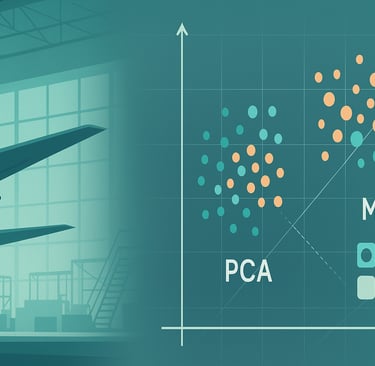
2. Meet the classics

Method Best suited for Core mathematics Outputs Typical libraries PCA (Principal Component Analysis) Continuous (numeric) variables Eigen-decomposition / SVD of the covariance matrix Principal components (orthogonal linear combinations) scikit-learn, numpy, statsmodels MCA (Multiple Correspondence Analysis) Categorical variables with multiple levels SVD of an indicator (one-hot) matrix, using a Chi-square metric Dimensions that maximize explained inertia of category profiles prince, R FactoMineR, Orange

(FAMD—Factor Analysis of Mixed Data—handles both in one framework.)

3. PCA in plain language

1. Standardize each continuous feature (mean 0, variance 1).

2. Compute covariance (or correlation) matrix.

3. Decompose it → eigenvectors = directions of maximum variance, eigenvalues = amount of variance they explain.

4. Project your data onto the top k eigenvectors to get a reduced data set.

Intuition: we rotate the coordinate system so the first axis points through the “fattest” part of the data cloud, the second through the next fattest, and so on.

4. MCA in plain language

1. One-hot encode each category level → a giant 0/1 “indicator matrix”.

2. Compute the matrix of relative frequencies and apply a Chi-square centering so that common categories don’t dominate.

3. Perform SVD on that matrix → principal dimensions (sometimes called “axes”) of association between categories.

4. Project individuals (rows) and categories (columns) into this lower-dimensional “association space”.

Intuition: categories that frequently co-occur are pulled together; rare or mutually exclusive categories are pushed apart.

5. How to handle different variable types

6. Practical tips & common pitfalls

7. Choosing between PCA and MCA (cheat sheet)

• All numeric? → PCA

• All categorical? → MCA

• Mixed? → FAMD or dual pipeline

• Goal = visual exploration → MCA biplots highlight which categories attract each other; PCA scatter-plots reveal numeric clusters.

• Goal = feed ML model → experiment: sometimes raw one-hot + standardization outperforms MCA; sometimes PCA components help shallow models generalize.

Key take-aways

1. Same family, different diet: both PCA and MCA are singular value decompositions—they just start from different distance metrics tailored to numeric vs categorical data.

2. Pre-processing is half the battle: scaling for PCA, sensible one-hot encoding and rare-level handling for MCA.

3. Interpretation differs: PCA components = weighted sums of original numbers; MCA axes = latent “themes” of category co-occurrence.

4. Don’t forget mixed solutions: FAMD or hybrid pipelines let you keep the flavor of both worlds without shoe-horning everything into numbers or categories.